Last updated on 2026-07-22
Jonathan Ho, Ajay Jain, Pieter Abbeel · NeurIPS 2020 · arXiv:2006.11239v2
阅读导航
论文定位与术语
这是一篇方法/算法论文。论证主线是:把固定 Gaussian 前向加噪过程与可学习反向链结合;用 ε 预测简化训练;以 CIFAR10/LSUN/CelebA-HQ 验证样本质量;再从率失真、自回归解码和插值解释模型的归纳偏置。
| Canonical term | 中文 | 使用约定 |
|---|---|---|
| diffusion probabilistic model / DDPM | 扩散概率模型 / 去噪扩散概率模型 | 首次全称,后用 DDPM |
| forward process | 前向过程(扩散过程) | 固定的逐步 Gaussian 加噪链 |
| reverse process | 反向过程 | 学习到的逐步去噪生成链 |
| variance schedule | 方差日程 | 保留符号 |
| noise prediction | 噪声预测 | 不译模型符号 |
| variational bound | 变分上界 | 与 ELBO/负对数似然语境保持一致 |
| denoising score matching | 去噪分数匹配 | 保持统一译名 |
| annealed Langevin dynamics | 退火 Langevin 动力学 | Langevin 保留英文 |
| bits/dim | 每维比特数 | 不改单位 |
逐页中英文对照
第 1 页
Source: p.1 S001
Original:
Denoising Diffusion Probabilistic Models Jonathan Ho UC Berkeley jonathanho@berkeley.edu Ajay Jain UC Berkeley ajayj@berkeley.edu Pieter Abbeel UC Berkeley pabbeel@cs.berkeley.edu Abstract We present high quality image synthesis results using diffusion probabilistic models, a class of latent variable models inspired by considerations from nonequilibrium thermodynamics. Our best results are obtained by training on a weighted variational bound designed according to a novel connection between diffusion probabilistic models and denoising score matching with Langevin dynamics, and our models naturally admit a progressive lossy decompression scheme that can be interpreted as a generalization of autoregressive decoding. On the unconditional CIFAR10 dataset, we obtain an Inception score of 9.46 and a state-of-the-art FID score of 3.17. On 256x256 LSUN, we obtain sample quality similar to ProgressiveGAN. Our implementation is available at https://github.com/hojonathanho/diffusion. 1 Introduction Deep generative models of all kinds have recently exhibited high quality samples in a wide variety of data modalities. Generative adversarial networks (GANs), autoregressive models, flows, and variational autoencoders (V AEs) have synthesized striking image and audio samples [ 14, 27, 3, 58, 38, 25, 10, 32, 44, 57, 26, 33, 45], and there have been remarkable advances in energy-based modeling and score matching that have produced images comparable to those of GANs [11, 55]. Figure 1: Generated samples on CelebA-HQ 256× 256 (left) and unconditional CIFAR10 (right) 34th Conference on Neural Information Processing Systems (NeurIPS 2020), Vancouver, Canada. arXiv:2006.11239v2 [cs.LG] 16 Dec 2020
中文:
摘要。 本文用扩散概率模型实现了高质量图像合成。该模型是一类受非平衡热力学启发的潜变量模型。作者提出一种加权变分下界训练方式,并揭示扩散模型与去噪分数匹配、Langevin 动力学之间的联系。模型还自然对应一种渐进式有损解压过程,可看作对自回归解码的推广。在无条件 CIFAR10 上,模型取得 Inception Score 9.46 和当时最优的 FID 3.17;在 256×256 LSUN 上,样本质量接近 ProgressiveGAN。
引言(本页)。 GAN、自回归模型、流模型和 VAE 已能生成高质量图像或音频,能量模型与分数匹配也取得明显进展。作者关注此前尚未被证明能生成高质量样本的扩散概率模型,并以 CelebA-HQ 与 CIFAR10 样本作为直观结果。
F001 · 图 1
Placed near: p.1 S001 Source: p.1
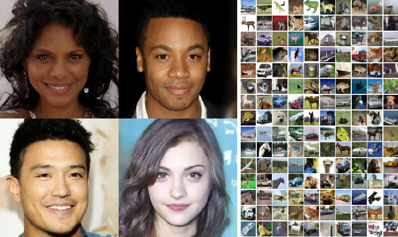
Original caption: Figure 1: Generated samples on CelebA-HQ 256×256 (left) and unconditional CIFAR10 (right)
中文图注: 图 1:CelebA-HQ 256×256(左)与无条件 CIFAR10(右)的生成样本。
Reading note: 首个直观证据:扩散模型已能在不同分辨率和数据分布上生成清晰、多样的样本。
第 2 页
Source: p.2 S002
Original:
Figure 2: The directed graphical model considered in this work. This paper presents progress in diffusion probabilistic models [53]. A diffusion probabilistic model (which we will call a “diffusion model” for brevity) is a parameterized Markov chain trained using variational inference to produce samples matching the data after finite time. Transitions of this chain are learned to reverse a diffusion process, which is a Markov chain that gradually adds noise to the data in the opposite direction of sampling until signal is destroyed. When the diffusion consists of small amounts of Gaussian noise, it is sufficient to set the sampling chain transitions to conditional Gaussians too, allowing for a particularly simple neural network parameterization. Diffusion models are straightforward to define and efficient to train, but to the best of our knowledge, there has been no demonstration that they are capable of generating high quality samples. We show that diffusion models actually are capable of generating high quality samples, sometimes better than the published results on other types of generative models (Section 4). In addition, we show that a certain parameterization of diffusion models reveals an equivalence with denoising score matching over multiple noise levels during training and with annealed Langevin dynamics during sampling (Section 3.2) [ 55, 61]. We obtained our best sample quality results using this parameterization (Section 4.2), so we consider this equivalence to be one of our primary contributions. Despite their sample quality, our models do not have competitive log likelihoods compared to other likelihood-based models (our models do, however, have log likelihoods better than the large estimates annealed importance sampling has been reported to produce for energy based models and score matching [11, 55]). We find that the majority of our models’ lossless codelengths are consumed to describe imperceptible image details (Section 4.3). We present a more refined analysis of this phenomenon in the language of lossy compression, and we show that the sampling procedure of diffusion models is a type of progressive decoding that resembles autoregressive decoding along a bit ordering that vastly generalizes what is normally possible with autoregressive models. 2 Background Diffusion models [53] are latent variable models of the form pθ(x0) := ∫ pθ(x0:T )dx1:T , where x1,..., xT are latents of the same dimensionality as the data x0∼ q(x0). The joint distribution pθ(x0:T ) is called the reverse process, and it is defined as a Markov chain with learned Gaussian transitions starting atp(xT ) =N (xT ; 0, I): pθ(x0:T ) :=p(xT ) T∏ t=1 pθ(xt−1|xt), p θ(xt−1|xt) :=N (xt−1; µθ(xt,t ), Σθ(xt,t )) (1) What distinguishes diffusion models from other types of latent variable models is that the approximate posteriorq(x1:T|x0), called the forward process or diffusion process, is fixed to a Markov chain that gradually adds Gaussian noise to the data according to a variance scheduleβ1,...,β T : q(x1:T|x0) := T∏ t=1 q(xt|xt−1), q (xt|xt−1) :=N (xt; √ 1−βtxt−1,βtI) (2) Training is performed by optimizing the usual variational bound on negative log likelihood: E [− logpθ(x0)]≤ Eq [ − log pθ(x0:T ) q(x1:T|x0) ] = Eq [ − logp(xT )− ∑ t≥1 logpθ(xt−1|xt) q(xt|xt−1) ] =:L (3) The forward process variances βt can be learned by reparameterization [ 33] or held constant as hyperparameters, and expressiveness of the reverse process is ensured in part by the choice of Gaussian conditionals inpθ(xt−1|xt), because both processes have the same functional form when βt are small [ 53]. A notable property of the forward process is that it admits sampling xt at an arbitrary timestept in closed form: using the notationαt := 1−βt and ¯αt :=∏t s=1αs, we have q(xt|x0) =N (xt;√¯αtx0, (1− ¯αt)I) (4) 2
中文:
扩散概率模型是一条用变分推断训练的参数化 Markov 链:前向链逐步向数据加入少量 Gaussian 噪声,直到信号被破坏;反向链学习撤销这一过程。由于每一步噪声很小,反向转移可用条件 Gaussian 分布表示,从而得到简洁的神经网络参数化。
本文的第一项核心贡献是证明扩散模型可以生成高质量样本。第二项贡献是:采用特定的反向过程参数化后,训练等价于跨多个噪声尺度的去噪分数匹配,采样则与退火 Langevin 动力学相联系。第三项贡献是从率失真角度解释似然与感知质量的差异,并把采样视为一种广义自回归式的渐进解码。
背景。 反向联合分布从标准 Gaussian 先验 出发,经学习到的 逐步生成 。前向近似后验 固定为按方差日程 加噪的 Markov 链。训练最小化负对数似然的变分上界。令 、,任意时刻的带噪样本可直接写为 ,因此训练无需逐步模拟全部前向链。
F002 · 图 2
Placed near: p.2 S002 Source: p.2
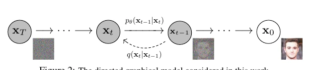
Original caption: Figure 2: The directed graphical model considered in this work.
中文图注: 图 2:本文研究的有向图模型。
Reading note: 从数据到噪声的前向链 q 固定;从噪声回到数据的反向链 pθ 由模型学习。
第 3 页
Source: p.3 S003
Original:
Efficient training is therefore possible by optimizing random terms of L with stochastic gradient descent. Further improvements come from variance reduction by rewritingL (3) as: Eq [ DKL(q(xT|x0)∥p(xT )) LT + ∑ t>1 DKL(q(xt−1|xt, x0)∥pθ(xt−1|xt)) Lt−1 − logpθ(x0|x1) L0 ] (5) (See Appendix A for details. The labels on the terms are used in Section 3.) Equation (5) uses KL divergence to directly comparepθ(xt−1|xt) against forward process posteriors, which are tractable when conditioned on x0: q(xt−1|xt, x0) =N (xt−1; ˜µt(xt, x0), ˜βtI), (6) where ˜µt(xt, x0) := √¯αt−1βt 1− ¯αt x0 + √αt(1− ¯αt−1) 1− ¯αt xt and ˜βt := 1− ¯αt−1 1− ¯αt βt (7) Consequently, all KL divergences in Eq. (5) are comparisons between Gaussians, so they can be calculated in a Rao-Blackwellized fashion with closed form expressions instead of high variance Monte Carlo estimates. 3 Diffusion models and denoising autoencoders Diffusion models might appear to be a restricted class of latent variable models, but they allow a large number of degrees of freedom in implementation. One must choose the variances βt of the forward process and the model architecture and Gaussian distribution parameterization of the reverse process. To guide our choices, we establish a new explicit connection between diffusion models and denoising score matching (Section 3.2) that leads to a simplified, weighted variational bound objective for diffusion models (Section 3.4). Ultimately, our model design is justified by simplicity and empirical results (Section 4). Our discussion is categorized by the terms of Eq. (5). 3.1 Forward process and LT We ignore the fact that the forward process variances βt are learnable by reparameterization and instead fix them to constants (see Section 4 for details). Thus, in our implementation, the approximate posteriorq has no learnable parameters, soLT is a constant during training and can be ignored. 3.2 Reverse process and L1:T−1 Now we discuss our choices inpθ(xt−1|xt) =N (xt−1; µθ(xt,t ), Σθ(xt,t )) for 1<t ≤T . First, we set Σθ(xt,t ) =σ2 t I to untrained time dependent constants. Experimentally, bothσ2 t =βt and σ2 t = ˜βt = 1−¯αt−1 1−¯αt βt had similar results. The first choice is optimal for x0∼N (0, I), and the second is optimal for x0 deterministically set to one point. These are the two extreme choices corresponding to upper and lower bounds on reverse process entropy for data with coordinatewise unit variance [53]. Second, to represent the mean µθ(xt,t ), we propose a specific parameterization motivated by the following analysis ofLt. Withpθ(xt−1|xt) =N (xt−1; µθ(xt,t ),σ 2 t I), we can write: Lt−1 = Eq [ 1 2σ2 t ∥˜µt(xt, x0)− µθ(xt,t )∥2 ] +C (8) whereC is a constant that does not depend onθ. So, we see that the most straightforward parameterization of µθ is a model that predicts ˜µt, the forward process posterior mean. However, we can expand Eq. (8) further by reparameterizing Eq. (4) as xt(x0, ϵ) =√¯αtx0 +√1− ¯αtϵ for ϵ∼N (0, I) and applying the forward process posterior formula (7): Lt−1−C = Ex0,ϵ [ 1 2σ2 t ˜µt ( xt(x0, ϵ), 1√¯αt (xt(x0, ϵ)− √ 1− ¯αtϵ) ) − µθ(xt(x0, ϵ),t ) 2] (9) = Ex0,ϵ [ 1 2σ2 t 1√αt ( xt(x0, ϵ)− βt√1− ¯αt ϵ ) − µθ(xt(x0, ϵ),t ) 2] (10) 3
中文:
将变分上界改写为式(5)后,它由终点先验匹配项 、逐步反向转移的 KL 项 和重建项 组成。给定 时,前向后验 是均值和方差均有闭式表达的 Gaussian 分布,因此各 KL 项都能以低方差的解析形式计算。
扩散模型与去噪自编码器。 模型设计需要确定前向方差日程、网络结构,以及反向 Gaussian 的均值和方差参数化。作者固定 ,使 成为训练常数;反向方差采用不训练的、随时间变化的各向同性常数。对均值而言,直接预测后验均值 是自然选择,但进一步重参数化后可让网络预测加入的噪声 。式(8)至(10)表明,这两种形式在数学上对应同一反向均值,而噪声预测会导向更简洁的目标。
第 4 页
Source: p.4 S004
Original:
Algorithm 1 Training 1: repeat 2: x0∼q(x0) 3: t∼ Uniform({1,...,T }) 4: ϵ∼N (0, I) 5: Take gradient descent step on ∇θ ϵ− ϵθ(√¯αtx0 +√1− ¯αtϵ,t ) 2 6: until converged Algorithm 2 Sampling 1: xT∼N (0, I) 2: fort =T,..., 1 do 3: z∼N (0, I) ift> 1, else z = 0 4: xt−1 = 1√αt ( xt− 1−αt√1−¯αt ϵθ(xt,t ) ) +σtz 5: end for 6: return x0 Equation (10) reveals that µθ must predict 1√αt ( xt− βt√1−¯αt ϵ ) given xt. Since xt is available as input to the model, we may choose the parameterization µθ(xt,t ) = ˜µt ( xt, 1√¯αt (xt− √ 1− ¯αtϵθ(xt)) ) = 1√αt ( xt− βt√1− ¯αt ϵθ(xt,t ) ) (11) where ϵθ is a function approximator intended to predict ϵ from xt. To sample xt−1∼pθ(xt−1|xt) is to compute xt−1 = 1√αt ( xt− βt√1−¯αt ϵθ(xt,t ) ) +σtz, where z∼N (0, I). The complete sampling procedure, Algorithm 2, resembles Langevin dynamics with ϵθ as a learned gradient of the data density. Furthermore, with the parameterization (11), Eq. (10) simplifies to: Ex0,ϵ [ β2 t 2σ2 tαt(1− ¯αt) ϵ− ϵθ(√¯αtx0 + √ 1− ¯αtϵ,t ) 2 ] (12) which resembles denoising score matching over multiple noise scales indexed byt [55]. As Eq. (12) is equal to (one term of) the variational bound for the Langevin-like reverse process (11), we see that optimizing an objective resembling denoising score matching is equivalent to using variational inference to fit the finite-time marginal of a sampling chain resembling Langevin dynamics. To summarize, we can train the reverse process mean function approximator µθ to predict ˜µt, or by modifying its parameterization, we can train it to predict ϵ. (There is also the possibility of predicting x0, but we found this to lead to worse sample quality early in our experiments.) We have shown that the ϵ-prediction parameterization both resembles Langevin dynamics and simplifies the diffusion model’s variational bound to an objective that resembles denoising score matching. Nonetheless, it is just another parameterization ofpθ(xt−1|xt), so we verify its effectiveness in Section 4 in an ablation where we compare predicting ϵ against predicting ˜µt. 3.3 Data scaling, reverse process decoder, and L0 We assume that image data consists of integers in{0, 1,..., 255} scaled linearly to [−1, 1]. This ensures that the neural network reverse process operates on consistently scaled inputs starting from the standard normal priorp(xT ). To obtain discrete log likelihoods, we set the last term of the reverse process to an independent discrete decoder derived from the GaussianN (x0; µθ(x1, 1),σ 2 1I): pθ(x0|x1) = D∏ i=1 ∫ δ+(xi 0) δ−(xi 0) N (x;µi θ(x1, 1),σ 2 1)dx δ+(x) = {∞ ifx = 1 x + 1 255 ifx< 1 δ−(x) = {−∞ ifx =−1 x− 1 255 ifx> −1 (13) where D is the data dimensionality and the i superscript indicates extraction of one coordinate. (It would be straightforward to instead incorporate a more powerful decoder like a conditional autoregressive model, but we leave that to future work.) Similar to the discretized continuous distributions used in V AE decoders and autoregressive models [34, 52], our choice here ensures that the variational bound is a lossless codelength of discrete data, without need of adding noise to the data or incorporating the Jacobian of the scaling operation into the log likelihood. At the end of sampling, we display µθ(x1, 1) noiselessly. 3.4 Simplified training objective With the reverse process and decoder defined above, the variational bound, consisting of terms derived from Eqs. (12) and (13), is clearly differentiable with respect toθ and is ready to be employed for 4
中文:
算法 1 每次随机采样数据 、时间步 与噪声 ,用均方误差训练网络从 预测噪声;算法 2 从 出发,逐步代入预测噪声并加入适当随机项,直到得到 。式(11)给出噪声预测到反向均值的映射,式(12)与多个噪声尺度上的去噪分数匹配具有相同形式,同时其采样更新类似 Langevin 动力学。
作者比较了预测 、预测 以及预测 ;早期实验中直接预测 的样本质量较差。数据像素从整数 线性缩放到 ,最后一步使用由 Gaussian 推导的独立离散解码器,使变分上界可解释为离散数据的无损码长。最终展示图像时使用 ,不再额外加噪。
A001 · 算法 1–2
Placed near: p.4 S004 Source: p.4
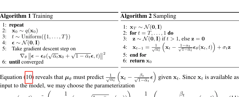
Original caption: Algorithms 1–2: Training and sampling.
中文图注: 算法 1–2:训练与采样。
Reading note: 训练随机抽取一个时间步预测噪声;采样必须依次执行反向步骤。
第 5 页
Source: p.5 S005
Original:
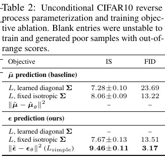
Table 1: CIFAR10 results. NLL measured in bits/dim. Model IS FID NLL Test (Train) Conditional EBM [11] 8.30 37 .9 JEM [17] 8.76 38 .4 BigGAN [3] 9.22 14 .73 StyleGAN2 + ADA (v1) [29] 10.06 2 .67 Unconditional Diffusion (original) [53] ≤ 5.40 Gated PixelCNN [59] 4.60 65 .93 3 .03 (2.90) Sparse Transformer [7] 2.80 PixelIQN [43] 5.29 49 .46 EBM [11] 6.78 38 .2 NCSNv2 [56] 31.75 NCSN [55] 8.87±0.12 25 .32 SNGAN [39] 8.22±0.05 21 .7 SNGAN-DDLS [4] 9.09±0.10 15 .42 StyleGAN2 + ADA (v1) [29] 9.74± 0.05 3 .26 Ours (L, fixed isotropicΣ) 7.67±0.13 13 .51 ≤ 3.70 (3.69) Ours (Lsimple) 9.46±0.11 3.17 ≤ 3.75 (3.72) Table 2: Unconditional CIFAR10 reverse process parameterization and training objective ablation. Blank entries were unstable to train and generated poor samples with out-ofrange scores. Objective IS FID ˜µ prediction (baseline) L, learned diagonal Σ 7.28±0.10 23 .69 L, fixed isotropicΣ 8.06±0.09 13 .22 ∥˜µ− ˜µθ∥2 – – ϵ prediction (ours) L, learned diagonal Σ – – L, fixed isotropicΣ 7.67±0.13 13 .51 ∥˜ϵ− ϵθ∥2 (Lsimple) 9.46±0.11 3 .17 training. However, we found it beneficial to sample quality (and simpler to implement) to train on the following variant of the variational bound: Lsimple(θ) := Et,x0,ϵ [ϵ− ϵθ(√¯αtx0 + √ 1− ¯αtϵ,t ) 2] (14) wheret is uniform between 1 andT . The t = 1 case corresponds to L0 with the integral in the discrete decoder definition (13) approximated by the Gaussian probability density function times the bin width, ignoringσ2 1 and edge effects. The t >1 cases correspond to an unweighted version of Eq. (12), analogous to the loss weighting used by the NCSN denoising score matching model [55]. (LT does not appear because the forward process variancesβt are fixed.) Algorithm 1 displays the complete training procedure with this simplified objective. Since our simplified objective (14) discards the weighting in Eq. (12), it is a weighted variational bound that emphasizes different aspects of reconstruction compared to the standard variational bound [18, 22]. In particular, our diffusion process setup in Section 4 causes the simplified objective to down-weight loss terms corresponding to smallt. These terms train the network to denoise data with very small amounts of noise, so it is beneficial to down-weight them so that the network can focus on more difficult denoising tasks at largert terms. We will see in our experiments that this reweighting leads to better sample quality. 4 Experiments We set T = 1000 for all experiments so that the number of neural network evaluations needed during sampling matches previous work [53, 55]. We set the forward process variances to constants increasing linearly from β1 = 10−4 to βT = 0.02. These constants were chosen to be small relative to data scaled to [−1, 1], ensuring that reverse and forward processes have approximately the same functional form while keeping the signal-to-noise ratio at xT as small as possible (LT = DKL(q(xT|x0)∥N (0, I))≈ 10−5 bits per dimension in our experiments). To represent the reverse process, we use a U-Net backbone similar to an unmasked PixelCNN++ [52, 48] with group normalization throughout [66]. Parameters are shared across time, which is specified to the network using the Transformer sinusoidal position embedding [60]. We use self-attention at the 16× 16 feature map resolution [63, 60]. Details are in Appendix B. 4.1 Sample quality Table 1 shows Inception scores, FID scores, and negative log likelihoods (lossless codelengths) on CIFAR10. With our FID score of 3.17, our unconditional model achieves better sample quality than most models in the literature, including class conditional models. Our FID score is computed with respect to the training set, as is standard practice; when we compute it with respect to the test set, the score is 5.24, which is still better than many of the training set FID scores in the literature. 5
中文:
作者没有直接使用带时间权重的完整变分上界,而采用式(14)的简化目标 :在均匀随机时间步上最小化真实噪声与预测噪声之间的均方误差。该目标降低了小 、低噪声且较容易的去噪项权重,使网络更多学习大 的困难去噪任务,实验表明这显著改善感知样本质量。
所有实验取 , 从 线性增加到 0.02。反向网络采用带 group normalization 的 U-Net/PixelCNN++ 风格骨干,用 Transformer 正弦位置编码注入时间步,并在 特征分辨率加入 self-attention。CIFAR10 上 模型达到 IS 9.46±0.11、FID 3.17;相对于测试集计算的 FID 为 5.24。完整变分下界带来更好码长,而简化目标带来更好样本质量。
T001 · 表 1
Placed near: p.5 S005 Source: p.5
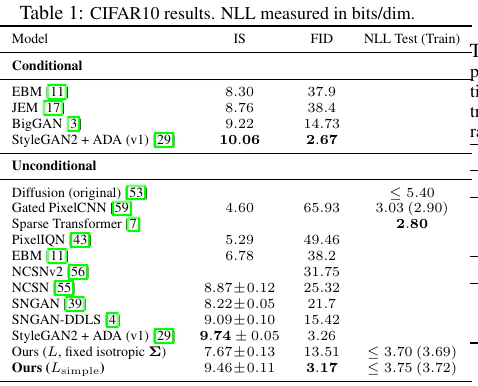
Original caption: Table 1: CIFAR10 results; NLL in bits/dim.
中文图注: 表 1:CIFAR10 结果,NLL 单位为 bits/dim。
Reading note: 重点比较无条件生成:Lsimple 达到 IS 9.46、FID 3.17,但 NLL 不是最优。
T002 · 表 2
Placed near: p.5 S005 Source: p.5
Original caption: Table 2: Reverse-process parameterization and objective ablation.
中文图注: 表 2:反向过程参数化与训练目标消融。
Reading note: ε 预测与简化目标组合显著优于其他稳定配置。
第 6 页
Source: p.6 S006
Original:
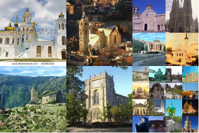
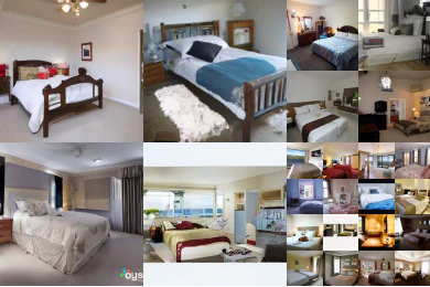
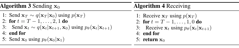
Figure 3: LSUN Church samples. FID=7.89 Figure 4: LSUN Bedroom samples. FID=4.90 Algorithm 3 Sending x0 1: Send xT∼q(xT|x0) usingp(xT ) 2: fort =T− 1,..., 2, 1 do 3: Send xt∼q(xt|xt+1, x0) usingpθ(xt|xt+1) 4: end for 5: Send x0 usingpθ(x0|x1) Algorithm 4 Receiving 1: Receive xT usingp(xT ) 2: fort =T− 1,..., 1, 0 do 3: Receive xt usingpθ(xt|xt+1) 4: end for 5: return x0 We find that training our models on the true variational bound yields better codelengths than training on the simplified objective, as expected, but the latter yields the best sample quality. See Fig. 1 for CIFAR10 and CelebA-HQ 256× 256 samples, Fig. 3 and Fig. 4 for LSUN 256× 256 samples [71], and Appendix D for more. 4.2 Reverse process parameterization and training objective ablation In Table 2, we show the sample quality effects of reverse process parameterizations and training objectives (Section 3.2). We find that the baseline option of predicting ˜µ works well only when trained on the true variational bound instead of unweighted mean squared error, a simplified objective akin to Eq. (14). We also see that learning reverse process variances (by incorporating a parameterized diagonal Σθ(xt) into the variational bound) leads to unstable training and poorer sample quality compared to fixed variances. Predicting ϵ, as we proposed, performs approximately as well as predicting ˜µ when trained on the variational bound with fixed variances, but much better when trained with our simplified objective. 4.3 Progressive coding Table 1 also shows the codelengths of our CIFAR10 models. The gap between train and test is at most 0.03 bits per dimension, which is comparable to the gaps reported with other likelihood-based models and indicates that our diffusion model is not overfitting (see Appendix D for nearest neighbor visualizations). Still, while our lossless codelengths are better than the large estimates reported for energy based models and score matching using annealed importance sampling [ 11], they are not competitive with other types of likelihood-based generative models [7]. Since our samples are nonetheless of high quality, we conclude that diffusion models have an inductive bias that makes them excellent lossy compressors. Treating the variational bound termsL1 +··· +LT as rate andL0 as distortion, our CIFAR10 model with the highest quality samples has a rate of 1.78 bits/dim and a distortion of 1.97 bits/dim, which amounts to a root mean squared error of 0.95 on a scale from 0 to 255. More than half of the lossless codelength describes imperceptible distortions. Progressive lossy compression We can probe further into the rate-distortion behavior of our model by introducing a progressive lossy code that mirrors the form of Eq. (5): see Algorithms 3 and 4, which assume access to a procedure, such as minimal random coding [19, 20], that can transmit a sample x∼q(x) using approximatelyDKL(q(x)∥p(x)) bits on average for any distributionsp and q, for which onlyp is available to the receiver beforehand. When applied tox0∼q(x0), Algorithms 3 and 4 transmitxT,..., x0 in sequence using a total expected codelength equal to Eq. (5). The receiver, 6
中文:
在 256×256 LSUN Church 与 Bedroom 上,模型分别达到 FID 7.89 与 4.90。消融实验显示:预测后验均值 只有配合真实变分上界时表现较好;学习反向方差会导致训练不稳定和样本质量下降;固定方差时,噪声预测与均值预测在完整上界下接近,但噪声预测配合 明显更优。
渐进编码。 CIFAR10 训练/测试码长差不超过 0.03 bits/dim,说明结果不是简单过拟合,但无损码长仍不及其他显式似然模型。作者提出关键解释:扩散模型具有有利于感知质量的归纳偏置,是优秀的有损压缩器。把 看作码率、把 看作失真,最佳样本模型的码率为 1.78 bits/dim、失真为 1.97 bits/dim,对应 标度下 RMSE 0.95;超过一半的无损码长用于描述肉眼难以感知的细节。算法 3/4 给出理论性的发送与接收过程。
F003 · 图 3
Placed near: p.6 S006 Source: p.6
Original caption: Figure 3: LSUN Church samples. FID=7.89.
中文图注: 图 3:LSUN Church 样本,FID=7.89。
Reading note: 观察场景结构与建筑多样性,同时注意部分样本仍带训练数据水印。
F004 · 图 4
Placed near: p.6 S006 Source: p.6
Original caption: Figure 4: LSUN Bedroom samples. FID=4.90.
中文图注: 图 4:LSUN Bedroom 样本,FID=4.90。
Reading note: 大模型在室内场景上取得较强 FID。
A002 · 算法 3–4
Placed near: p.6 S006 Source: p.6
Original caption: Algorithms 3–4: Sending and receiving x0.
中文图注: 算法 3–4:渐进发送与接收 x0。
Reading note: 这是变分上界的理论编码解释,并非可直接部署的高维压缩器。
第 7 页
Source: p.7 S007
Original:
at any timet, has the partial information xt fully available and can progressively estimate: x0≈ ˆx0 = ( xt− √ 1− ¯αtϵθ(xt) ) /√¯αt (15) due to Eq. (4). (A stochastic reconstruction x0∼ pθ(x0|xt) is also valid, but we do not consider it here because it makes distortion more difficult to evaluate.) Figure 5 shows the resulting ratedistortion plot on the CIFAR10 test set. At each timet, the distortion is calculated as the root mean squared error √ ∥x0− ˆx0∥2/D, and the rate is calculated as the cumulative number of bits received so far at time t. The distortion decreases steeply in the low-rate region of the rate-distortion plot, indicating that the majority of the bits are indeed allocated to imperceptible distortions. 0 200 400 600 800 1,000 0 20 40 60 80 Reverse process steps (T−t) Distortion (RMSE) 0 200 400 600 800 1,000 0 0.5 1 1.5 Reverse process steps (T−t) Rate (bits/dim) 0 0.5 1 1.5 0 20 40 60 80 Rate (bits/dim) Distortion (RMSE) Figure 5: Unconditional CIFAR10 test set rate-distortion vs. time. Distortion is measured in root mean squared error on a [0, 255] scale. See Table 4 for details. Progressive generation We also run a progressive unconditional generation process given by progressive decompression from random bits. In other words, we predict the result of the reverse process, ˆx0, while sampling from the reverse process using Algorithm 2. Figures 6 and 10 show the resulting sample quality of ˆx0 over the course of the reverse process. Large scale image features appear first and details appear last. Figure 7 shows stochastic predictionsx0∼pθ(x0|xt) with xt frozen for varioust. Whent is small, all but fine details are preserved, and whent is large, only large scale features are preserved. Perhaps these are hints of conceptual compression [18]. Figure 6: Unconditional CIFAR10 progressive generation (ˆx0 over time, from left to right). Extended samples and sample quality metrics over time in the appendix (Figs. 10 and 14). Figure 7: When conditioned on the same latent, CelebA-HQ 256× 256 samples share high-level attributes. Bottom-right quadrants are xt, and other quadrants are samples frompθ(x0|xt). Connection to autoregressive decoding Note that the variational bound (5) can be rewritten as: L =DKL(q(xT )∥p(xT )) + Eq [∑ t≥1 DKL(q(xt−1|xt)∥pθ(xt−1|xt)) ] +H(x0) (16) (See Appendix A for a derivation.) Now consider setting the diffusion process length T to the dimensionality of the data, defining the forward process so thatq(xt|x0) places all probability mass on x0 with the firstt coordinates masked out (i.e.q(xt|xt−1) masks out thetth coordinate), setting p(xT ) to place all mass on a blank image, and, for the sake of argument, taking pθ(xt−1|xt) to 7
中文:
在渐进式有损解压中,接收者获得中间变量 后即可由式(15)估计原图。CIFAR10 的率失真曲线表明,在极低码率区失真迅速下降,随后大量比特只改善几乎不可见的细节。
渐进生成也呈现从粗到细的结构:反向过程早期先确定大尺度形状,后期再补充纹理细节。固定同一中间潜变量后,多次随机解码在较小 时仅细节不同,在较大 时只保留性别、姿态、发色等高层属性,这暗示中间状态包含分层语义。
作者进一步把变分上界改写成式(16),说明若前向过程逐坐标遮挡、反向过程逐坐标恢复,训练就退化为自回归模型。因此 Gaussian 扩散可理解为采用连续噪声与广义“比特顺序”的自回归模型;其顺序不是简单的像素排列。
F005 · 图 5
Placed near: p.7 S007 Source: p.7

Original caption: Figure 5: CIFAR10 rate–distortion over reverse time.
中文图注: 图 5:CIFAR10 反向时间上的率失真关系。
Reading note: 低码率区失真快速下降,之后大量码长只改善细微、难感知的误差。
F006 · 图 6
Placed near: p.7 S007 Source: p.7
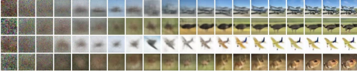
Original caption: Figure 6: CIFAR10 progressive generation.
中文图注: 图 6:CIFAR10 渐进生成。
Reading note: 从左到右先出现大尺度轮廓,再逐步增加纹理与类别细节。
F007 · 图 7
Placed near: p.7 S007 Source: p.7
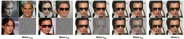
Original caption: Figure 7: Samples conditioned on shared CelebA-HQ intermediate latents.
中文图注: 图 7:共享 CelebA-HQ 中间潜变量的条件样本。
Reading note: 同一中间状态保留高层属性,而后续随机性主要改变细节。
第 8 页
Source: p.8 S008
Original:
Figure 8: Interpolations of CelebA-HQ 256x256 images with 500 timesteps of diffusion. be a fully expressive conditional distribution. With these choices, DKL(q(xT )∥p(xT )) = 0, and minimizingDKL(q(xt−1|xt)∥pθ(xt−1|xt)) trainspθ to copy coordinatest + 1,...,T unchanged and to predict thetth coordinate givent + 1,...,T . Thus, trainingpθ with this particular diffusion is training an autoregressive model. We can therefore interpret the Gaussian diffusion model (2) as a kind of autoregressive model with a generalized bit ordering that cannot be expressed by reordering data coordinates. Prior work has shown that such reorderings introduce inductive biases that have an impact on sample quality [38], so we speculate that the Gaussian diffusion serves a similar purpose, perhaps to greater effect since Gaussian noise might be more natural to add to images compared to masking noise. Moreover, the Gaussian diffusion length is not restricted to equal the data dimension; for instance, we useT = 1000, which is less than the dimension of the 32× 32× 3 or 256× 256× 3 images in our experiments. Gaussian diffusions can be made shorter for fast sampling or longer for model expressiveness. 4.4 Interpolation We can interpolate source images x0, x′ 0∼ q(x0) in latent space using q as a stochastic encoder, xt, x′ t∼q(xt|x0), then decoding the linearly interpolated latent ¯xt = (1−λ)x0 +λx′ 0 into image space by the reverse process, ¯x0 ∼ p(x0|¯xt). In effect, we use the reverse process to remove artifacts from linearly interpolating corrupted versions of the source images, as depicted in Fig. 8 (left). We fixed the noise for different values of λ so xt and x′ t remain the same. Fig. 8 (right) shows interpolations and reconstructions of original CelebA-HQ 256× 256 images (t = 500). The reverse process produces high-quality reconstructions, and plausible interpolations that smoothly vary attributes such as pose, skin tone, hairstyle, expression and background, but not eyewear. Larger t results in coarser and more varied interpolations, with novel samples att = 1000 (Appendix Fig. 9). 5 Related Work While diffusion models might resemble flows [ 9, 46, 10, 32, 5, 16, 23] and V AEs [33, 47, 37], diffusion models are designed so thatq has no parameters and the top-level latent xT has nearly zero mutual information with the data x0. Our ϵ-prediction reverse process parameterization establishes a connection between diffusion models and denoising score matching over multiple noise levels with annealed Langevin dynamics for sampling [55, 56]. Diffusion models, however, admit straightforward log likelihood evaluation, and the training procedure explicitly trains the Langevin dynamics sampler using variational inference (see Appendix C for details). The connection also has the reverse implication that a certain weighted form of denoising score matching is the same as variational inference to train a Langevin-like sampler. Other methods for learning transition operators of Markov chains include infusion training [2], variational walkback [15], generative stochastic networks [1], and others [50, 54, 36, 42, 35, 65]. By the known connection between score matching and energy-based modeling, our work could have implications for other recent work on energy-based models [67–69, 12, 70, 13, 11, 41, 17, 8]. Our rate-distortion curves are computed over time in one evaluation of the variational bound, reminiscent of how rate-distortion curves can be computed over distortion penalties in one run of annealed importance sampling [24]. Our progressive decoding argument can be seen in convolutional DRAW and related models [ 18, 40] and may also lead to more general designs for subscale orderings or sampling strategies for autoregressive models [38, 64]. 8
中文:
Gaussian 扩散提供了一种比坐标遮挡更适合图像的归纳偏置,并允许通过改变 在采样速度与模型表达能力之间权衡。
插值。 作者先把两幅图像扩散到同一噪声层级,在潜空间进行线性混合,再由反向过程去除线性混合带来的伪影。 时,插值会平滑改变姿态、肤色、发型、表情和背景,但眼镜属性不一定连续;更大的 产生更粗粒度、更多样的插值, 时几乎成为新样本。
相关工作。 与 flow 和 VAE 不同,扩散模型的前向过程无可学习参数,顶层潜变量 与数据几乎无互信息。其噪声预测形式连接了去噪分数匹配与退火 Langevin 采样,但扩散模型还能直接计算似然,并通过变分推断显式训练有限步采样器。作者也把该框架与能量模型、Markov 转移学习、渐进解码和自回归子尺度顺序联系起来。
F008 · 图 8
Placed near: p.8 S008 Source: p.8
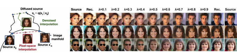
Original caption: Figure 8: CelebA-HQ interpolation after 500 diffusion steps.
中文图注: 图 8:扩散 500 步后的 CelebA-HQ 插值。
Reading note: 反向过程将噪声空间线性混合映射为平滑且逼真的语义过渡。
第 9 页
Source: p.9 S009
Original:
6 Conclusion We have presented high quality image samples using diffusion models, and we have found connections among diffusion models and variational inference for training Markov chains, denoising score matching and annealed Langevin dynamics (and energy-based models by extension), autoregressive models, and progressive lossy compression. Since diffusion models seem to have excellent inductive biases for image data, we look forward to investigating their utility in other data modalities and as components in other types of generative models and machine learning systems. Broader Impact Our work on diffusion models takes on a similar scope as existing work on other types of deep generative models, such as efforts to improve the sample quality of GANs, flows, autoregressive models, and so forth. Our paper represents progress in making diffusion models a generally useful tool in this family of techniques, so it may serve to amplify any impacts that generative models have had (and will have) on the broader world. Unfortunately, there are numerous well-known malicious uses of generative models. Sample generation techniques can be employed to produce fake images and videos of high profile figures for political purposes. While fake images were manually created long before software tools were available, generative models such as ours make the process easier. Fortunately, CNN-generated images currently have subtle flaws that allow detection [ 62], but improvements in generative models may make this more difficult. Generative models also reflect the biases in the datasets on which they are trained. As many large datasets are collected from the internet by automated systems, it can be difficult to remove these biases, especially when the images are unlabeled. If samples from generative models trained on these datasets proliferate throughout the internet, then these biases will only be reinforced further. On the other hand, diffusion models may be useful for data compression, which, as data becomes higher resolution and as global internet traffic increases, might be crucial to ensure accessibility of the internet to wide audiences. Our work might contribute to representation learning on unlabeled raw data for a large range of downstream tasks, from image classification to reinforcement learning, and diffusion models might also become viable for creative uses in art, photography, and music. Acknowledgments and Disclosure of Funding This work was supported by ONR PECASE and the NSF Graduate Research Fellowship under grant number DGE-1752814. Google’s TensorFlow Research Cloud (TFRC) provided Cloud TPUs. References [1] Guillaume Alain, Yoshua Bengio, Li Yao, Jason Yosinski, Eric Thibodeau-Laufer, Saizheng Zhang, and Pascal Vincent. GSNs: generative stochastic networks. Information and Inference: A Journal of the IMA , 5(2):210–249, 2016. [2] Florian Bordes, Sina Honari, and Pascal Vincent. Learning to generate samples from noise through infusion training. In International Conference on Learning Representations , 2017. [3] Andrew Brock, Jeff Donahue, and Karen Simonyan. Large scale GAN training for high fidelity natural image synthesis. In International Conference on Learning Representations , 2019. [4] Tong Che, Ruixiang Zhang, Jascha Sohl-Dickstein, Hugo Larochelle, Liam Paull, Yuan Cao, and Yoshua Bengio. Your GAN is secretly an energy-based model and you should use discriminator driven latent sampling. arXiv preprint arXiv:2003.06060, 2020. [5] Tian Qi Chen, Yulia Rubanova, Jesse Bettencourt, and David K Duvenaud. Neural ordinary differential equations. In Advances in Neural Information Processing Systems , pages 6571–6583, 2018. [6] Xi Chen, Nikhil Mishra, Mostafa Rohaninejad, and Pieter Abbeel. PixelSNAIL: An improved autoregressive generative model. In International Conference on Machine Learning , pages 863–871, 2018. [7] Rewon Child, Scott Gray, Alec Radford, and Ilya Sutskever. Generating long sequences with sparse transformers. arXiv preprint arXiv:1904.10509, 2019. 9
中文:
结论。 本文证明扩散模型可以生成高质量图像,并统一联系了:用于训练 Markov 链的变分推断、去噪分数匹配、退火 Langevin 动力学、能量模型、自回归模型与渐进式有损压缩。作者认为扩散过程对图像具有良好归纳偏置,值得扩展到其他数据模态和生成系统。
更广泛影响。 扩散模型与其他深度生成模型一样,既可能促进压缩、无监督表征学习和艺术创作,也可能降低制造虚假图像/视频的门槛,并复制、放大互联网训练数据中的偏见。随着生成质量提高,现有检测伪造内容的方法也可能更难奏效。
致谢部分说明研究由 ONR PECASE、NSF Graduate Research Fellowship 与 Google TFRC Cloud TPU 支持。参考文献条目从本页开始。
第 10 页
Source: p.10 S010
Original:
[8] Yuntian Deng, Anton Bakhtin, Myle Ott, Arthur Szlam, and Marc’Aurelio Ranzato. Residual energy-based models for text generation. arXiv preprint arXiv:2004.11714, 2020. [9] Laurent Dinh, David Krueger, and Yoshua Bengio. NICE: Non-linear independent components estimation. arXiv preprint arXiv:1410.8516, 2014. [10] Laurent Dinh, Jascha Sohl-Dickstein, and Samy Bengio. Density estimation using Real NVP. arXiv preprint arXiv:1605.08803, 2016. [11] Yilun Du and Igor Mordatch. Implicit generation and modeling with energy based models. In Advances in Neural Information Processing Systems, pages 3603–3613, 2019. [12] Ruiqi Gao, Yang Lu, Junpei Zhou, Song-Chun Zhu, and Ying Nian Wu. Learning generative ConvNets via multi-grid modeling and sampling. In Proceedings of the IEEE Conference on Computer Vision and Pattern Recognition, pages 9155–9164, 2018. [13] Ruiqi Gao, Erik Nijkamp, Diederik P Kingma, Zhen Xu, Andrew M Dai, and Ying Nian Wu. Flow contrastive estimation of energy-based models. In Proceedings of the IEEE/CVF Conference on Computer Vision and Pattern Recognition, pages 7518–7528, 2020. [14] Ian Goodfellow, Jean Pouget-Abadie, Mehdi Mirza, Bing Xu, David Warde-Farley, Sherjil Ozair, Aaron Courville, and Yoshua Bengio. Generative adversarial nets. In Advances in Neural Information Processing Systems, pages 2672–2680, 2014. [15] Anirudh Goyal, Nan Rosemary Ke, Surya Ganguli, and Yoshua Bengio. Variational walkback: Learning a transition operator as a stochastic recurrent net. In Advances in Neural Information Processing Systems , pages 4392–4402, 2017. [16] Will Grathwohl, Ricky T. Q. Chen, Jesse Bettencourt, and David Duvenaud. FFJORD: Free-form continuous dynamics for scalable reversible generative models. In International Conference on Learning Representations, 2019. [17] Will Grathwohl, Kuan-Chieh Wang, Joern-Henrik Jacobsen, David Duvenaud, Mohammad Norouzi, and Kevin Swersky. Your classifier is secretly an energy based model and you should treat it like one. In International Conference on Learning Representations , 2020. [18] Karol Gregor, Frederic Besse, Danilo Jimenez Rezende, Ivo Danihelka, and Daan Wierstra. Towards conceptual compression. In Advances In Neural Information Processing Systems , pages 3549–3557, 2016. [19] Prahladh Harsha, Rahul Jain, David McAllester, and Jaikumar Radhakrishnan. The communication complexity of correlation. In Twenty-Second Annual IEEE Conference on Computational Complexity (CCC’07), pages 10–23. IEEE, 2007. [20] Marton Havasi, Robert Peharz, and José Miguel Hernández-Lobato. Minimal random code learning: Getting bits back from compressed model parameters. In International Conference on Learning Representations, 2019. [21] Martin Heusel, Hubert Ramsauer, Thomas Unterthiner, Bernhard Nessler, and Sepp Hochreiter. GANs trained by a two time-scale update rule converge to a local Nash equilibrium. In Advances in Neural Information Processing Systems, pages 6626–6637, 2017. [22] Irina Higgins, Loic Matthey, Arka Pal, Christopher Burgess, Xavier Glorot, Matthew Botvinick, Shakir Mohamed, and Alexander Lerchner. beta-V AE: Learning basic visual concepts with a constrained variational framework. In International Conference on Learning Representations , 2017. [23] Jonathan Ho, Xi Chen, Aravind Srinivas, Yan Duan, and Pieter Abbeel. Flow++: Improving flow-based generative models with variational dequantization and architecture design. In International Conference on Machine Learning, 2019. [24] Sicong Huang, Alireza Makhzani, Yanshuai Cao, and Roger Grosse. Evaluating lossy compression rates of deep generative models. In International Conference on Machine Learning , 2020. [25] Nal Kalchbrenner, Aaron van den Oord, Karen Simonyan, Ivo Danihelka, Oriol Vinyals, Alex Graves, and Koray Kavukcuoglu. Video pixel networks. In International Conference on Machine Learning , pages 1771–1779, 2017. [26] Nal Kalchbrenner, Erich Elsen, Karen Simonyan, Seb Noury, Norman Casagrande, Edward Lockhart, Florian Stimberg, Aaron van den Oord, Sander Dieleman, and Koray Kavukcuoglu. Efficient neural audio synthesis. In International Conference on Machine Learning , pages 2410–2419, 2018. [27] Tero Karras, Timo Aila, Samuli Laine, and Jaakko Lehtinen. Progressive growing of GANs for improved quality, stability, and variation. In International Conference on Learning Representations , 2018. [28] Tero Karras, Samuli Laine, and Timo Aila. A style-based generator architecture for generative adversarial networks. In Proceedings of the IEEE Conference on Computer Vision and Pattern Recognition , pages 10
中文:
本页为参考文献续页。为保证作者、题名、会议/期刊与页码的可检索性,条目保持英文原貌,不逐条翻译。
第 11 页
Source: p.11 S011
Original:
4401–4410, 2019. [29] Tero Karras, Miika Aittala, Janne Hellsten, Samuli Laine, Jaakko Lehtinen, and Timo Aila. Training generative adversarial networks with limited data. arXiv preprint arXiv:2006.06676v1, 2020. [30] Tero Karras, Samuli Laine, Miika Aittala, Janne Hellsten, Jaakko Lehtinen, and Timo Aila. Analyzing and improving the image quality of StyleGAN. In Proceedings of the IEEE/CVF Conference on Computer Vision and Pattern Recognition, pages 8110–8119, 2020. [31] Diederik P Kingma and Jimmy Ba. Adam: A method for stochastic optimization. In International Conference on Learning Representations, 2015. [32] Diederik P Kingma and Prafulla Dhariwal. Glow: Generative flow with invertible 1x1 convolutions. In Advances in Neural Information Processing Systems , pages 10215–10224, 2018. [33] Diederik P Kingma and Max Welling. Auto-encoding variational Bayes. arXiv preprint arXiv:1312.6114, 2013. [34] Diederik P Kingma, Tim Salimans, Rafal Jozefowicz, Xi Chen, Ilya Sutskever, and Max Welling. Improved variational inference with inverse autoregressive flow. In Advances in Neural Information Processing Systems, pages 4743–4751, 2016. [35] John Lawson, George Tucker, Bo Dai, and Rajesh Ranganath. Energy-inspired models: Learning with sampler-induced distributions. In Advances in Neural Information Processing Systems , pages 8501–8513, 2019. [36] Daniel Levy, Matt D. Hoffman, and Jascha Sohl-Dickstein. Generalizing Hamiltonian Monte Carlo with neural networks. In International Conference on Learning Representations , 2018. [37] Lars Maaløe, Marco Fraccaro, Valentin Liévin, and Ole Winther. BIV A: A very deep hierarchy of latent variables for generative modeling. In Advances in Neural Information Processing Systems , pages 6548–6558, 2019. [38] Jacob Menick and Nal Kalchbrenner. Generating high fidelity images with subscale pixel networks and multidimensional upscaling. In International Conference on Learning Representations , 2019. [39] Takeru Miyato, Toshiki Kataoka, Masanori Koyama, and Yuichi Yoshida. Spectral normalization for generative adversarial networks. In International Conference on Learning Representations , 2018. [40] Alex Nichol. VQ-DRAW: A sequential discrete V AE. arXiv preprint arXiv:2003.01599, 2020. [41] Erik Nijkamp, Mitch Hill, Tian Han, Song-Chun Zhu, and Ying Nian Wu. On the anatomy of MCMC-based maximum likelihood learning of energy-based models. arXiv preprint arXiv:1903.12370, 2019. [42] Erik Nijkamp, Mitch Hill, Song-Chun Zhu, and Ying Nian Wu. Learning non-convergent non-persistent short-run MCMC toward energy-based model. In Advances in Neural Information Processing Systems , pages 5233–5243, 2019. [43] Georg Ostrovski, Will Dabney, and Remi Munos. Autoregressive quantile networks for generative modeling. In International Conference on Machine Learning , pages 3936–3945, 2018. [44] Ryan Prenger, Rafael Valle, and Bryan Catanzaro. WaveGlow: A flow-based generative network for speech synthesis. In ICASSP 2019-2019 IEEE International Conference on Acoustics, Speech and Signal Processing (ICASSP), pages 3617–3621. IEEE, 2019. [45] Ali Razavi, Aaron van den Oord, and Oriol Vinyals. Generating diverse high-fidelity images with VQ- V AE-2. InAdvances in Neural Information Processing Systems , pages 14837–14847, 2019. [46] Danilo Rezende and Shakir Mohamed. Variational inference with normalizing flows. In International Conference on Machine Learning, pages 1530–1538, 2015. [47] Danilo Jimenez Rezende, Shakir Mohamed, and Daan Wierstra. Stochastic backpropagation and approximate inference in deep generative models. In International Conference on Machine Learning , pages 1278–1286, 2014. [48] Olaf Ronneberger, Philipp Fischer, and Thomas Brox. U-Net: Convolutional networks for biomedical image segmentation. In International Conference on Medical Image Computing and Computer-Assisted Intervention, pages 234–241. Springer, 2015. [49] Tim Salimans and Durk P Kingma. Weight normalization: A simple reparameterization to accelerate training of deep neural networks. In Advances in Neural Information Processing Systems , pages 901–909, 2016. [50] Tim Salimans, Diederik Kingma, and Max Welling. Markov Chain Monte Carlo and variational inference: Bridging the gap. In International Conference on Machine Learning , pages 1218–1226, 2015. 11
中文:
本页为参考文献续页。条目保持英文原貌。
第 12 页
Source: p.12 S012
Original:
[51] Tim Salimans, Ian Goodfellow, Wojciech Zaremba, Vicki Cheung, Alec Radford, and Xi Chen. Improved techniques for training gans. In Advances in Neural Information Processing Systems , pages 2234–2242, 2016. [52] Tim Salimans, Andrej Karpathy, Xi Chen, and Diederik P Kingma. PixelCNN++: Improving the PixelCNN with discretized logistic mixture likelihood and other modifications. In International Conference on Learning Representations, 2017. [53] Jascha Sohl-Dickstein, Eric Weiss, Niru Maheswaranathan, and Surya Ganguli. Deep unsupervised learning using nonequilibrium thermodynamics. In International Conference on Machine Learning , pages 2256–2265, 2015. [54] Jiaming Song, Shengjia Zhao, and Stefano Ermon. A-NICE-MC: Adversarial training for MCMC. In Advances in Neural Information Processing Systems , pages 5140–5150, 2017. [55] Yang Song and Stefano Ermon. Generative modeling by estimating gradients of the data distribution. In Advances in Neural Information Processing Systems , pages 11895–11907, 2019. [56] Yang Song and Stefano Ermon. Improved techniques for training score-based generative models. arXiv preprint arXiv:2006.09011, 2020. [57] Aaron van den Oord, Sander Dieleman, Heiga Zen, Karen Simonyan, Oriol Vinyals, Alex Graves, Nal Kalchbrenner, Andrew Senior, and Koray Kavukcuoglu. WaveNet: A generative model for raw audio. arXiv preprint arXiv:1609.03499, 2016. [58] Aaron van den Oord, Nal Kalchbrenner, and Koray Kavukcuoglu. Pixel recurrent neural networks. International Conference on Machine Learning , 2016. [59] Aaron van den Oord, Nal Kalchbrenner, Oriol Vinyals, Lasse Espeholt, Alex Graves, and Koray Kavukcuoglu. Conditional image generation with PixelCNN decoders. In Advances in Neural Information Processing Systems, pages 4790–4798, 2016. [60] Ashish Vaswani, Noam Shazeer, Niki Parmar, Jakob Uszkoreit, Llion Jones, Aidan N Gomez, Łukasz Kaiser, and Illia Polosukhin. Attention is all you need. In Advances in Neural Information Processing Systems, pages 5998–6008, 2017. [61] Pascal Vincent. A connection between score matching and denoising autoencoders. Neural Computation, 23(7):1661–1674, 2011. [62] Sheng-Yu Wang, Oliver Wang, Richard Zhang, Andrew Owens, and Alexei A Efros. Cnn-generated images are surprisingly easy to spot...for now. In Proceedings of the IEEE Conference on Computer Vision and Pattern Recognition, 2020. [63] Xiaolong Wang, Ross Girshick, Abhinav Gupta, and Kaiming He. Non-local neural networks. In Proceedings of the IEEE Conference on Computer Vision and Pattern Recognition , pages 7794–7803, 2018. [64] Auke J Wiggers and Emiel Hoogeboom. Predictive sampling with forecasting autoregressive models. arXiv preprint arXiv:2002.09928, 2020. [65] Hao Wu, Jonas Köhler, and Frank Noé. Stochastic normalizing flows. arXiv preprint arXiv:2002.06707, 2020. [66] Yuxin Wu and Kaiming He. Group normalization. InProceedings of the European Conference on Computer Vision (ECCV), pages 3–19, 2018. [67] Jianwen Xie, Yang Lu, Song-Chun Zhu, and Yingnian Wu. A theory of generative convnet. InInternational Conference on Machine Learning, pages 2635–2644, 2016. [68] Jianwen Xie, Song-Chun Zhu, and Ying Nian Wu. Synthesizing dynamic patterns by spatial-temporal generative convnet. In Proceedings of the IEEE Conference on Computer Vision and Pattern Recognition , pages 7093–7101, 2017. [69] Jianwen Xie, Zilong Zheng, Ruiqi Gao, Wenguan Wang, Song-Chun Zhu, and Ying Nian Wu. Learning descriptor networks for 3d shape synthesis and analysis. In Proceedings of the IEEE Conference on Computer Vision and Pattern Recognition, pages 8629–8638, 2018. [70] Jianwen Xie, Song-Chun Zhu, and Ying Nian Wu. Learning energy-based spatial-temporal generative convnets for dynamic patterns. IEEE Transactions on Pattern Analysis and Machine Intelligence , 2019. [71] Fisher Yu, Yinda Zhang, Shuran Song, Ari Seff, and Jianxiong Xiao. LSUN: Construction of a large-scale image dataset using deep learning with humans in the loop. arXiv preprint arXiv:1506.03365, 2015. [72] Sergey Zagoruyko and Nikos Komodakis. Wide residual networks. arXiv preprint arXiv:1605.07146 , 2016. 12
中文:
本页为参考文献末页。条目保持英文原貌。
第 13 页
Source: p.13 S013
Original:
Extra information LSUN FID scores for LSUN datasets are included in Table 3. Scores marked with∗ are reported by StyleGAN2 as baselines, and other scores are reported by their respective authors. Table 3: FID scores for LSUN 256× 256 datasets Model LSUN Bedroom LSUN Church LSUN Cat ProgressiveGAN [27] 8.34 6.42 37.52 StyleGAN [28] 2.65 4.21∗ 8.53∗ StyleGAN2 [30] - 3.86 6.93 Ours (Lsimple) 6.36 7.89 19.75 Ours (Lsimple, large) 4.90 - - Progressive compression Our lossy compression argument in Section 4.3 is only a proof of concept, because Algorithms 3 and 4 depend on a procedure such as minimal random coding [20], which is not tractable for high dimensional data. These algorithms serve as a compression interpretation of the variational bound (5) of Sohl-Dickstein et al. [53], not yet as a practical compression system. Table 4: Unconditional CIFAR10 test set rate-distortion values (accompanies Fig. 5) Reverse process time (T−t + 1) Rate (bits/dim) Distortion (RMSE [0, 255]) 1000 1.77581 0.95136 900 0.11994 12.02277 800 0.05415 18.47482 700 0.02866 24.43656 600 0.01507 30.80948 500 0.00716 38.03236 400 0.00282 46.12765 300 0.00081 54.18826 200 0.00013 60.97170 100 0.00000 67.60125 A Extended derivations Below is a derivation of Eq. (5), the reduced variance variational bound for diffusion models. This material is from Sohl-Dickstein et al. [53]; we include it here only for completeness. L = Eq [ − log pθ(x0:T ) q(x1:T|x0) ] (17) = Eq − logp(xT )− ∑ t≥1 logpθ(xt−1|xt) q(xt|xt−1) (18) = Eq [ − logp(xT )− ∑ t>1 logpθ(xt−1|xt) q(xt|xt−1) − logpθ(x0|x1) q(x1|x0) ] (19) = Eq [ − logp(xT )− ∑ t>1 log pθ(xt−1|xt) q(xt−1|xt, x0)· q(xt−1|x0) q(xt|x0) − logpθ(x0|x1) q(x1|x0) ] (20) = Eq [ − log p(xT ) q(xT|x0)− ∑ t>1 log pθ(xt−1|xt) q(xt−1|xt, x0)− logpθ(x0|x1) ] (21) 13
中文:
补充结果给出 LSUN 256×256 的 FID:本文模型在 Bedroom、Church、Cat 上分别报告 4.90(大模型)、7.89、19.75。作者明确指出渐进压缩仍只是概念验证,因为算法 3/4 依赖高维情况下不可行的最小随机编码;它目前是对变分上界的压缩解释,而非实用编码系统。表 4 给出 CIFAR10 各反向时间点的码率与 RMSE。
附录 A。 式(17)至(22)把原始变分目标逐步改写为终点先验 KL、逐步后验 KL 与重建负对数似然之和,即正文式(5)。这些推导沿用 Sohl-Dickstein 等人的结果,本文为完整性而列出。
T003 · 表 3
Placed near: p.13 S013 Source: p.13
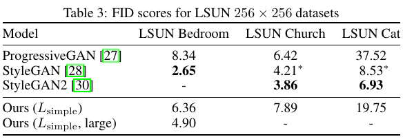
Original caption: Table 3: LSUN 256×256 FID scores.
中文图注: 表 3:LSUN 256×256 的 FID。
Reading note: DDPM 当时接近强 GAN 基线,但并非所有 LSUN 类别都领先。
T004 · 表 4
Placed near: p.13 S013 Source: p.13
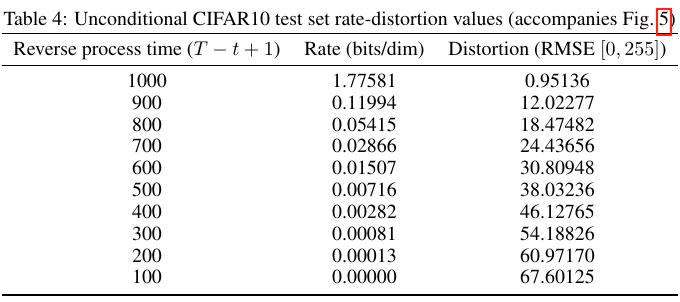
Original caption: Table 4: CIFAR10 rate–distortion values.
中文图注: 表 4:CIFAR10 率失真数值。
Reading note: 反向步骤增加时码率上升、RMSE 下降;收益高度不均匀。
第 14 页
Source: p.14 S014
Original:
= Eq [ DKL(q(xT|x0)∥p(xT )) + ∑ t>1 DKL(q(xt−1|xt, x0)∥pθ(xt−1|xt))− logpθ(x0|x1) ] (22) The following is an alternate version of L. It is not tractable to estimate, but it is useful for our discussion in Section 4.3. L = Eq − logp(xT )− ∑ t≥1 logpθ(xt−1|xt) q(xt|xt−1) (23) = Eq − logp(xT )− ∑ t≥1 logpθ(xt−1|xt) q(xt−1|xt) · q(xt−1) q(xt) (24) = Eq − logp(xT ) q(xT )− ∑ t≥1 logpθ(xt−1|xt) q(xt−1|xt) − logq(x0) (25) =DKL(q(xT )∥p(xT )) + Eq ∑ t≥1 DKL(q(xt−1|xt)∥pθ(xt−1|xt)) +H(x0) (26) B Experimental details Our neural network architecture follows the backbone of PixelCNN++ [52], which is a U-Net [48] based on a Wide ResNet [72]. We replaced weight normalization [49] with group normalization [66] to make the implementation simpler. Our 32× 32 models use four feature map resolutions (32× 32 to 4× 4), and our 256× 256 models use six. All models have two convolutional residual blocks per resolution level and self-attention blocks at the 16× 16 resolution between the convolutional blocks [6]. Diffusion timet is specified by adding the Transformer sinusoidal position embedding [60] into each residual block. Our CIFAR10 model has 35.7 million parameters, and our LSUN and CelebA-HQ models have 114 million parameters. We also trained a larger variant of the LSUN Bedroom model with approximately 256 million parameters by increasing filter count. We used TPU v3-8 (similar to 8 V100 GPUs) for all experiments. Our CIFAR model trains at 21 steps per second at batch size 128 (10.6 hours to train to completion at 800k steps), and sampling a batch of 256 images takes 17 seconds. Our CelebA-HQ/LSUN (256 2) models train at 2.2 steps per second at batch size 64, and sampling a batch of 128 images takes 300 seconds. We trained on CelebA-HQ for 0.5M steps, LSUN Bedroom for 2.4M steps, LSUN Cat for 1.8M steps, and LSUN Church for 1.2M steps. The larger LSUN Bedroom model was trained for 1.15M steps. Apart from an initial choice of hyperparameters early on to make network size fit within memory constraints, we performed the majority of our hyperparameter search to optimize for CIFAR10 sample quality, then transferred the resulting settings over to the other datasets: • We chose the βt schedule from a set of constant, linear, and quadratic schedules, all constrained so that LT ≈ 0. We set T = 1000 without a sweep, and we chose a linear schedule fromβ1 = 10−4 toβT = 0.02. • We set the dropout rate on CIFAR10 to0.1 by sweeping over the values{0.1, 0.2, 0.3, 0.4}. Without dropout on CIFAR10, we obtained poorer samples reminiscent of the overfitting artifacts in an unregularized PixelCNN++ [52]. We set dropout rate on the other datasets to zero without sweeping. • We used random horizontal flips during training for CIFAR10; we tried training both with and without flips, and found flips to improve sample quality slightly. We also used random horizontal flips for all other datasets except LSUN Bedroom. • We tried Adam [31] and RMSProp early on in our experimentation process and chose the former. We left the hyperparameters to their standard values. We set the learning rate to 2× 10⁻⁴ without any sweeping, and we lowered it to 2× 10⁻⁵ for the 256× 256 images, which seemed unstable to train with the larger learning rate. 14
中文:
式(23)至(26)给出另一种不可直接估计、但有助于解释渐进编码的目标分解:它由聚合后验与先验的 KL、各步反向条件分布的 KL,以及数据熵 构成。
附录 B:实验细节。 网络沿用 PixelCNN++ 的 Wide-ResNet U-Net 骨干,以 group normalization 替代 weight normalization;32×32 模型采用 4 个分辨率层级,256×256 模型采用 6 个,每层两组卷积残差块,并在 16×16 分辨率插入 self-attention。CIFAR10 模型 35.7M 参数,LSUN/CelebA-HQ 模型 114M,Bedroom 大模型约 256M。训练使用 TPU v3-8;CIFAR10 完成 800k 步约 10.6 小时,生成 256 张图约 17 秒;256×256 模型生成 128 张图约 300 秒。超参数主要在 CIFAR10 上选择后迁移到其他数据集。
第 15 页
Source: p.15 S015
Original:
• We set the batch size to 128 for CIFAR10 and 64 for larger images. We did not sweep over these values. • We used EMA on model parameters with a decay factor of 0.9999. We did not sweep over this value. Final experiments were trained once and evaluated throughout training for sample quality. Sample quality scores and log likelihood are reported on the minimum FID value over the course of training. On CIFAR10, we calculated Inception and FID scores on 50000 samples using the original code from the OpenAI [ 51] and TTUR [ 21] repositories, respectively. On LSUN, we calculated FID scores on 50000 samples using code from the StyleGAN2 [30] repository. CIFAR10 and CelebA-HQ were loaded as provided by TensorFlow Datasets ( https://www.tensorflow.org/datasets), and LSUN was prepared using code from StyleGAN. Dataset splits (or lack thereof) are standard from the papers that introduced their usage in a generative modeling context. All details can be found in the source code release. C Discussion on related work Our model architecture, forward process definition, and prior differ from NCSN [55, 56] in subtle but important ways that improve sample quality, and, notably, we directly train our sampler as a latent variable model rather than adding it after training post-hoc. In greater detail:
- We use a U-Net with self-attention; NCSN uses a RefineNet with dilated convolutions. We condition all layers ont by adding in the Transformer sinusoidal position embedding, rather than only in normalization layers (NCSNv1) or only at the output (v2).
- Diffusion models scale down the data with each forward process step (by a√1−βt factor) so that variance does not grow when adding noise, thus providing consistently scaled inputs to the neural net reverse process. NCSN omits this scaling factor.
- Unlike NCSN, our forward process destroys signal (DKL(q(xT|x0)∥N (0, I))≈ 0), ensuring a close match between the prior and aggregate posterior of xT . Also unlike NCSN, our βt are very small, which ensures that the forward process is reversible by a Markov chain with conditional Gaussians. Both of these factors prevent distribution shift when sampling.
- Our Langevin-like sampler has coefficients (learning rate, noise scale, etc.) derived rigorously from βt in the forward process. Thus, our training procedure directly trains our sampler to match the data distribution afterT steps: it trains the sampler as a latent variable model using variational inference. In contrast, NCSN’s sampler coefficients are set by hand post-hoc, and their training procedure is not guaranteed to directly optimize a quality metric of their sampler. D Samples Additional samples Figure 11, 13, 16, 17, 18, and 19 show uncurated samples from the diffusion models trained on CelebA-HQ, CIFAR10 and LSUN datasets. Latent structure and reverse process stochasticity During sampling, both the prior xT ∼ N (0, I) and Langevin dynamics are stochastic. To understand the significance of the second source of noise, we sampled multiple images conditioned on the same intermediate latent for the CelebA 256× 256 dataset. Figure 7 shows multiple draws from the reverse process x0∼ pθ(x0|xt) that share the latent xt fort∈{ 1000, 750, 500, 250}. To accomplish this, we run a single reverse chain from an initial draw from the prior. At the intermediate timesteps, the chain is split to sample multiple images. When the chain is split after the prior draw at xT=1000, the samples differ significantly. However, when the chain is split after more steps, samples share high-level attributes like gender, hair color, eyewear, saturation, pose and facial expression. This indicates that intermediate latents like x750 encode these attributes, despite their imperceptibility. Coarse-to-fine interpolation Figure 9 shows interpolations between a pair of source CelebA 256× 256 images as we vary the number of diffusion steps prior to latent space interpolation. Increasing the number of diffusion steps destroys more structure in the source images, which the 15
中文:
训练批量为 CIFAR10 128、较大图像 64;参数 EMA 衰减 0.9999。最终实验只训练一次,并在训练期间持续评估,报告最低 FID 时的样本质量与似然。CIFAR10 的 IS/FID、LSUN 的 FID 均基于 50,000 个样本和公开实现。
附录 C:与 NCSN 的差异。 DDPM 使用带 self-attention 的 U-Net,并在所有残差块注入时间编码;前向过程每步同时缩放信号,避免加噪导致方差增长;终点分布被设计为接近标准 Gaussian,且步长足够小,以减少采样时的分布偏移;Langevin 式采样器的步长与噪声系数由 严格推导,并作为潜变量模型通过变分推断端到端训练,而非训练后手工设置。
附录 D。 补充图展示未筛选样本、最近邻、渐进生成和潜变量结构。固定中间潜变量后再分叉采样表明:越晚分叉,样本越共享高层属性,证明中间状态编码了不可直接看见但有语义的结构。
第 16 页
Source: p.16 S016
Original:
model completes during the reverse process. This allows us to interpolate at both fine granularities and coarse granularities. In the limiting case of 0 diffusion steps, the interpolation mixes source images in pixel space. On the other hand, after 1000 diffusion steps, source information is lost and interpolations are novel samples. SourceRec.λ=0.1λ=0.2λ=0.3λ=0.4λ=0.5λ=0.6λ=0.7λ=0.8λ=0.9Rec.Source 1000 steps 875 steps 750 steps 625 steps 500 steps 375 steps 250 steps 125 steps 0 steps Figure 9: Coarse-to-fine interpolations that vary the number of diffusion steps prior to latent mixing. 0 200 400 600 800 1,000 2 4 6 8 10 Reverse process steps (T−t) Inception Score 0 200 400 600 800 1,000 0 100 200 300 Reverse process steps (T−t) FID Figure 10: Unconditional CIFAR10 progressive sampling quality over time 16
中文:
粗到细插值实验改变潜变量混合前的扩散步数:0 步等价于像素空间混合;步数增加时,源图结构被逐渐破坏,再由反向过程补全,因此可以控制插值的细粒度与粗粒度;1000 步时源信息基本消失,插值成为新样本。图 10 同时显示渐进采样过程中 IS 上升、FID 下降,定量支持“先形成全局结构、后完善细节”的观察。
F009 · 图 9
Placed near: p.16 S016 Source: p.16
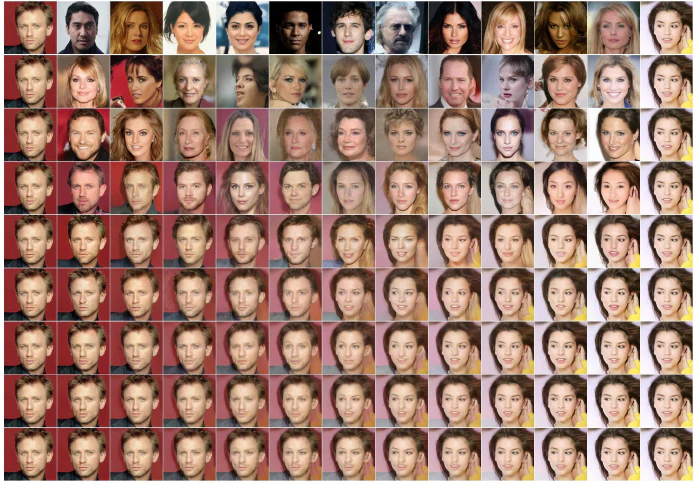
Original caption: Figure 9: Coarse-to-fine interpolation.
中文图注: 图 9:从粗到细的插值。
Reading note: 扩散步数控制源图信息保留程度:0 步偏像素混合,1000 步接近新生成。
F010 · 图 10
Placed near: p.16 S016 Source: p.16
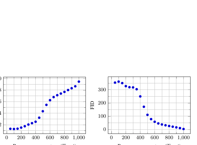
Original caption: Figure 10: CIFAR10 progressive sampling quality over time.
中文图注: 图 10:CIFAR10 渐进采样质量随时间变化。
Reading note: 反向过程推进时 IS 上升、FID 下降,量化了逐步成像过程。
补充图与表
以下图像来自仅含补充可视化的第 17–25 页。
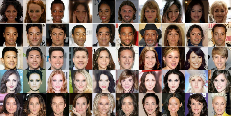
F011 · p.17
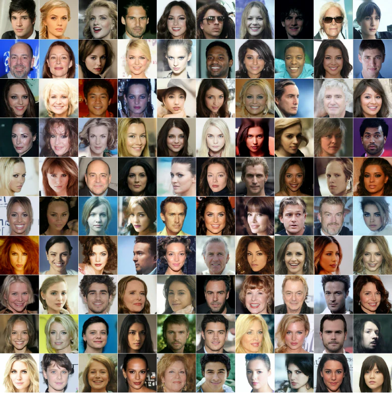
Original caption: Figure 11: CelebA-HQ 256×256 generated samples.
中文图注: 图 11:CelebA-HQ 256×256 生成样本。
Reading note: 用于检查样本多样性与人脸细节。
F012A · p.18
Original caption: Figure 12a: Pixel-space nearest neighbors.
中文图注: 图 12a:像素空间最近邻。
Reading note: 生成样本位于最左列,其余为训练集最近邻,用于排查复制。
F012B · p.18
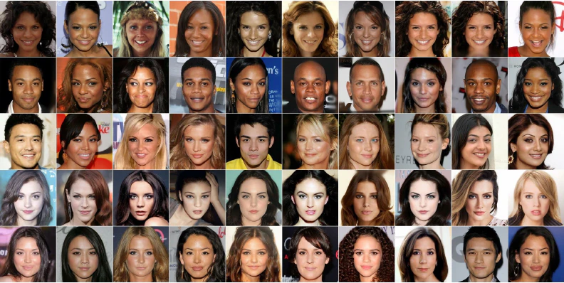
Original caption: Figure 12b: Inception-feature nearest neighbors.
中文图注: 图 12b:Inception 特征空间最近邻。
Reading note: 语义相近并不等于像素复制;两种距离共同支持非记忆化判断。
F013 · p.19
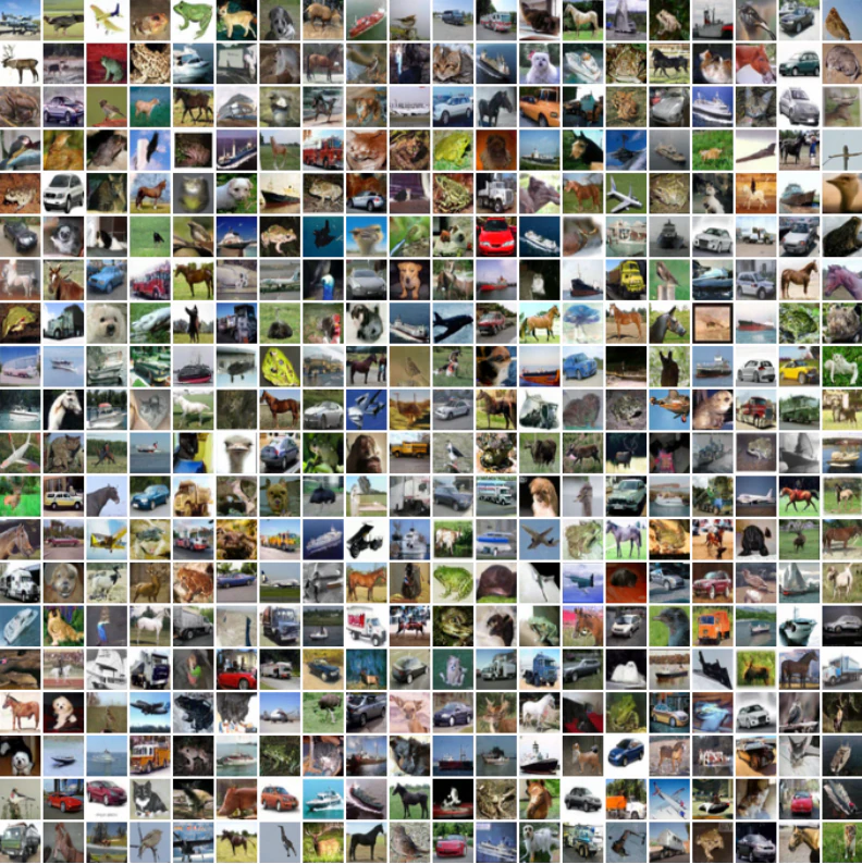
Original caption: Figure 13: Unconditional CIFAR10 generated samples.
中文图注: 图 13:无条件 CIFAR10 生成样本。
Reading note: 未筛选样本展示类别覆盖与局部失败模式。
F014 · p.20
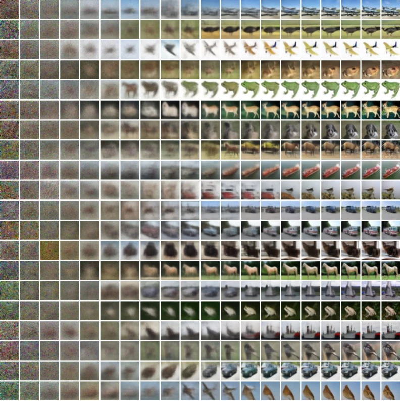
Original caption: Figure 14: Unconditional CIFAR10 progressive generation.
中文图注: 图 14:无条件 CIFAR10 渐进生成。
Reading note: 扩展版轨迹再次显示轮廓先于纹理形成。
F015A · p.21
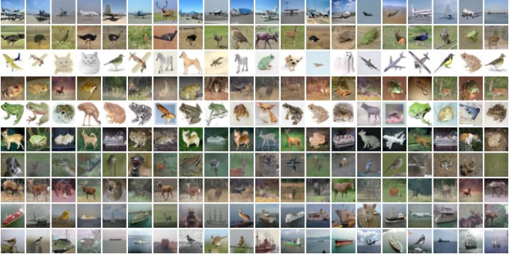
Original caption: Figure 15a: CIFAR10 pixel-space nearest neighbors.
中文图注: 图 15a:CIFAR10 像素空间最近邻。
Reading note: 用于检查训练样本记忆。
F015B · p.21
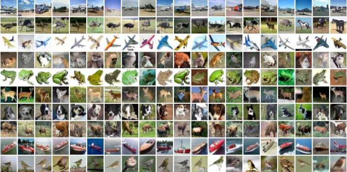
Original caption: Figure 15b: CIFAR10 Inception-feature nearest neighbors.
中文图注: 图 15b:CIFAR10 Inception 特征最近邻。
Reading note: 对比语义邻近样本,未见逐像素复制。
F016 · p.22
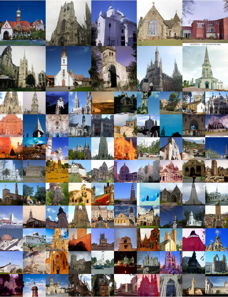
Original caption: Figure 16: LSUN Church generated samples. FID=7.89.
中文图注: 图 16:LSUN Church 生成样本,FID=7.89。
Reading note: 扩展未筛选样本用于观察覆盖范围和结构错误。
F017 · p.23
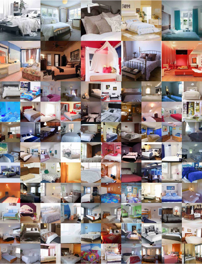
Original caption: Figure 17: LSUN Bedroom samples, large model. FID=4.90.
中文图注: 图 17:LSUN Bedroom 大模型样本,FID=4.90。
Reading note: 大模型样本整体更清晰,但仍存在布局不一致。
F018 · p.24
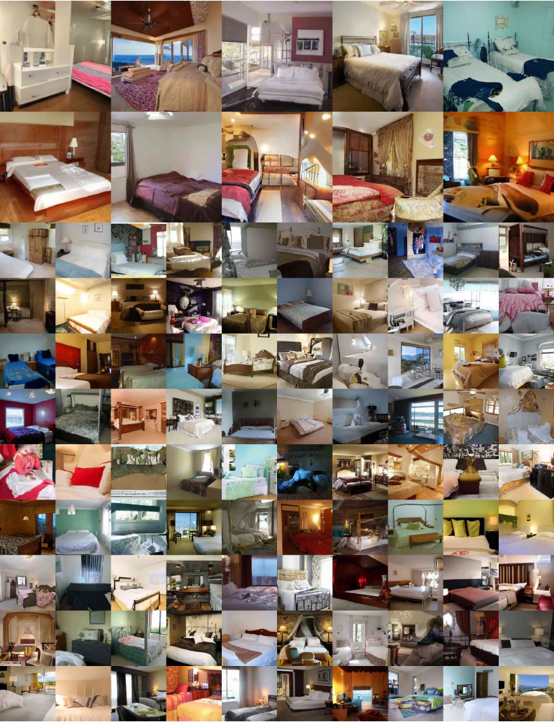
Original caption: Figure 18: LSUN Bedroom samples, small model. FID=6.36.
中文图注: 图 18:LSUN Bedroom 小模型样本,FID=6.36。
Reading note: 与大模型对照可见容量提升带来的质量收益。
F019 · p.25
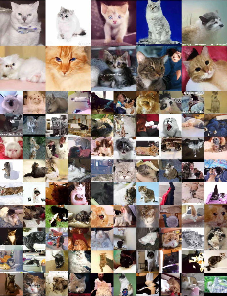
Original caption: Figure 19: LSUN Cat generated samples. FID=19.75.
中文图注: 图 19:LSUN Cat 生成样本,FID=19.75。
Reading note: 复杂姿态和背景使该类别明显难于 Bedroom/Church。
批判性精读
- 真正的算法突破是参数化与目标的组合。 扩散 Markov 链并非本文首次提出;DDPM 的关键是把反向均值改写为 ε 预测,并用无时间权重的 训练,从而把可实现性转化为高样本质量。
- 高感知质量与高似然不是同一目标。 完整变分上界改善码长,简化目标改善 FID。率失真分析说明,似然会为肉眼难辨的细节分配大量容量。
- 计算成本是核心边界。 原始方法需要 1000 次串行网络求值;附录给出的 256×256 采样速度远慢于一次前馈生成,这后来成为加速采样研究的主要问题。
- 压缩解释主要是概念性的。 作者在附录明确承认渐进编码依赖高维不可行的最小随机编码,不能把它误读为当时已经可用的压缩系统。
- 实验结论需按时代语境理解。 CIFAR10 FID=3.17 是 2020 年的重要结果,但表 3 表明 LSUN 上并未全面超越 StyleGAN2;论文的长期影响更多来自统一框架与可扩展训练目标。
- 更广泛影响判断仍然有效。 生成内容滥用、训练数据偏见与检测难度会随模型能力同步增加。